
The aim is to find a way to automate the drawing of the bounding boxes around the potential meteor echoes on the spectrograms, reducing or even eliminating the need for manual labeling of spectrograms.
The resulting bounding boxes may then be used in the Radio Meteor Zoo (RMZ), to be validated and/or corrected by volunteers.
More information about the RMZ can be found here and [Calders, 2017].
In an attempt to achieve human-like performance on the detection of meteor echoes on spectrograms, the use of convolutional neural networks (CNN) is explored.
This choice was made as CNNs are inherently good at looking at parts of multi-dimensional data such as images individually.
This leads them to be the most prominent machine learning method whenever locality in the data must be taken into account.
Like most machine learning methods, NNs need labeled training data, and this is where the dataset from the RMZ comes into play.
The questions which will be explored are the following:
-
Is it possible to develop a technique using convolutional neural networks which achieves human-like performance for the detection of meteor echoes on the (labeled) spectrograms provided by the BRAMS network?
- Given that meteor echoes can be highly irregular in shape, is it possible to use per-pixel predictions?
- How can these per-pixel predictions be used to generate meaningful bounding boxes?
-
How can the results of the technique be evaluated?
- How does one compare bounding boxes?
- Given a similarity metric for bounding boxes, how similar do these have to be?
- How does one analyze the precision and recall of the method?
All software has been written in Python 3 using the Tensorflow framework.
MSc thesis of Stan Draulans (2019)
By training a convolutional neural network on a sliding window over labeled spectrograms, the model developed by Draulans is able to generate pixel regions of high confidence where meteor echoes occur.
These regions can then be identified using a series of post-processing steps, such as blurring and thresholding, after which bounding boxes can be calculated for these regions.
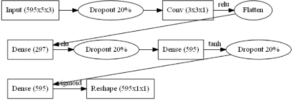
Vertical slice network architecture
Evaluating the quality of these generated bounding boxes is no simple matter.
As the labeled training data produced by the aggregation of labelings by volunteers often included parts of the background around the actual meteor echoes,
the generated bounding boxes are often rather small compared to the reference.
When trying to evaluate whether a generated bounding box is similar enough to the reference, this becomes a hindering factor as a similarity threshold must be set.
This similarity threshold forms the basis for the metrics used to measure the model performance on a per bounding box level, and therefore clearly has a significant influence on the perceived performance of the model.
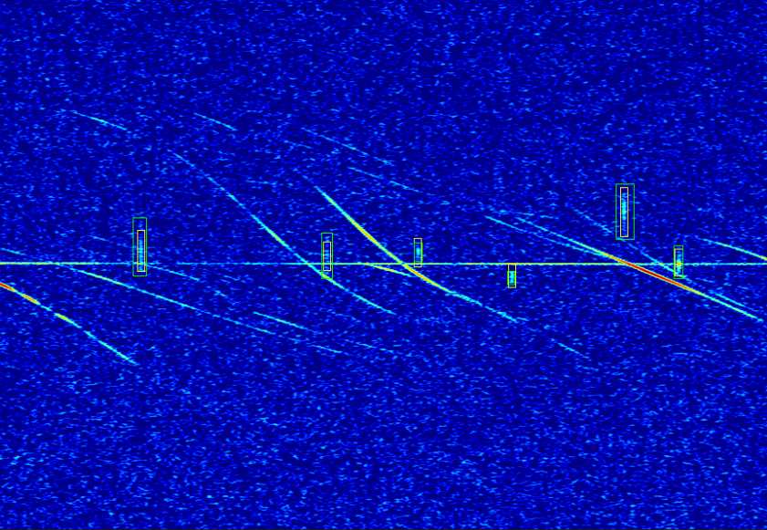
The bounding box predictions (in yellow) and the target bounding boxes (in green).
Therefore, in an attempt to bypass the bias introduced by this similarity threshold, the model was validated by experts on a limited set of unseen spectrograms, yielding a precision score of 0.852, a recall score of 0.676 and a F1-score of 0.754.
This precision is rather good, but the recall could be improved.
Research performed by Jean Lobet (2021)
Lobet studied three different types of CNNs:
- A simple CNN that makes use of alternance of convolution layers and max pooling.
- A transposed CNN, where the data is upsampled by a learned kernel.
- A dilated CNN, which is a technique that expands the kernel (input) by inserting holes between its consecutive elements.
In simpler terms, it is the same as simple convolution but it involves pixel skipping, so as to cover a larger area of the input. It avoids loss of resolution of the output image.
The loss function used in the training is the Mean Squared Logarithmic Error (MSLE). As the MSLE penalizes more underpredictions than overpredictions, it seemed rather suited as the target is sparse.
Simple CNN
This model makes use of alternance of convolution layers and (max) pooling. The main idea behind a pooling layer is to “accumulate” features from maps generated by convolving a filter over an image.
Formally, its function is to progressively reduce the spatial size of the representation to reduce the amount of parameters and computation in the network. The use of pooling between the convolution allows the following convolution layers to leverage more and more contextual information.
The second part of the model reconstruct the images based on the high dimensional shrinked image
Transposed CNN
The main idea behind the transposed convolution is to embed the upsampling procedure within the convolution. The data is no more upsampled by static kernels but rather by a learned one.
Dilated CNN
In [Yu & Koltun, 2016], the authors describe how they get rid of pooling by using growing dilated convolution. They were able to achieve higher resolution segmentation (owing the removal of pooling) as well as higher quality segmentation.
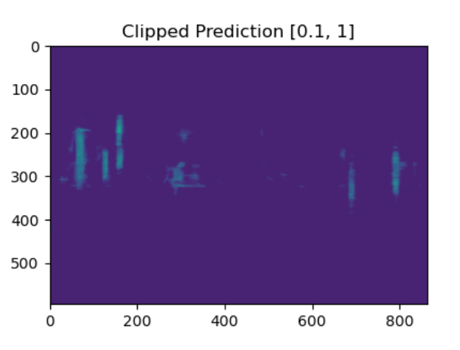
Comparison between methods
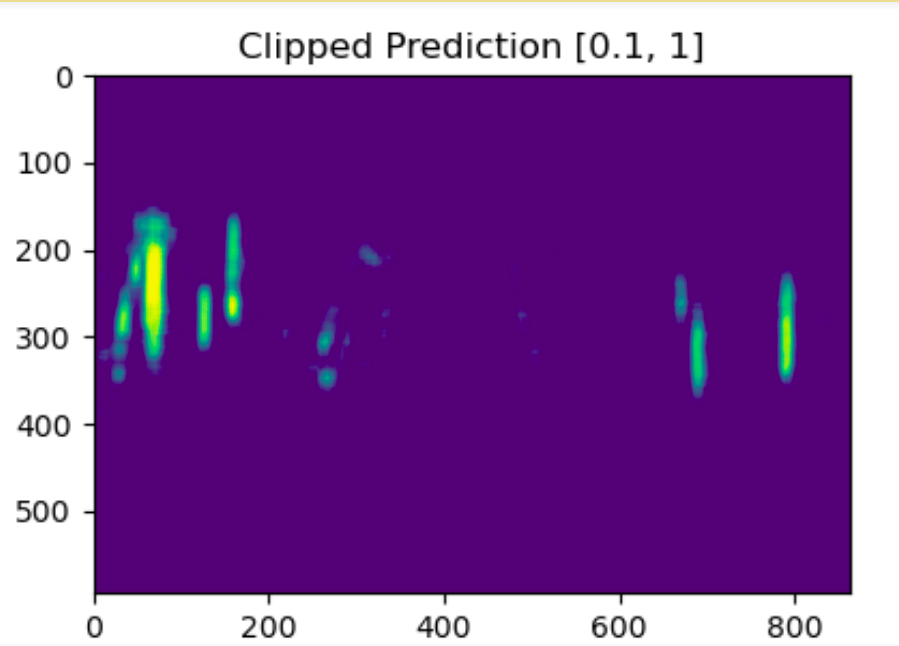
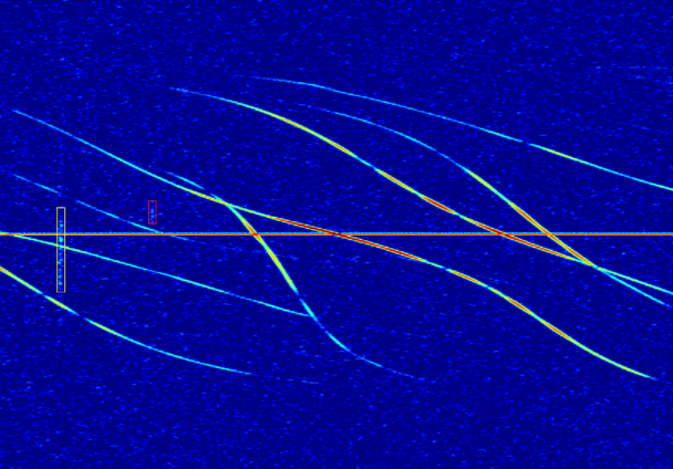
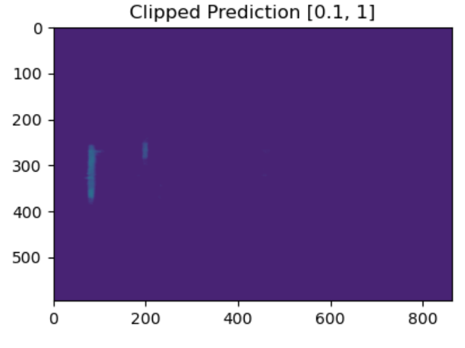
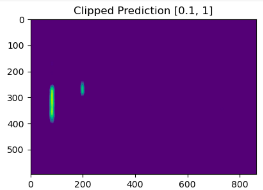
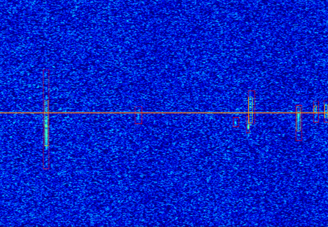
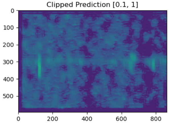
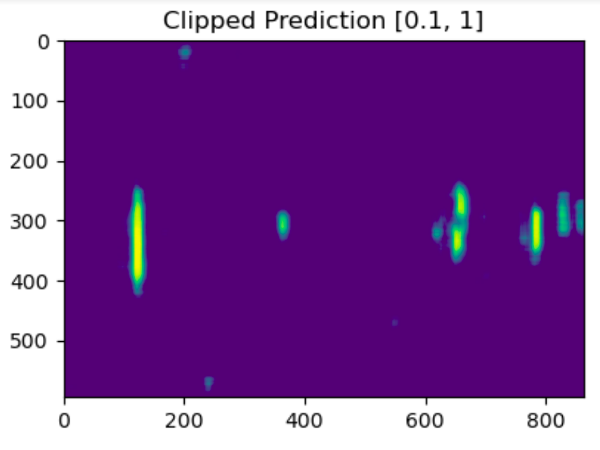
False detection of military airplanes
Draulans’ method:
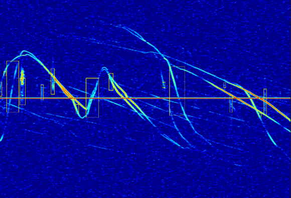
Lobet’s SimpleCNN:
Lobet's TransposedCNN:
![]()
Lobet's DilatedCNN:
Low intensity underdense meteor trails
Draulans’ method:
Lobet’s SimpleCNN:
Lobet's TransposedCNN:
![]()
Lobet's DilatedCNN:
Noisy spectrograms
Draulans’ method:
Lobet’s SimpleCNN:
Lobet's TransposedCNN:
![]()
Lobet's DilatedCNN:
Summary
| Draulans | Lobet SimpleCNN | Lobet TransposedCNN | Lobet DilatedCNN | |
| precision | 0.852 | 0.831 | 0.755 | 0.861 |
| recall | 0.676 | 0.820 | 0.873 | 0.879 |
| F1 | 0.754 | 0.826 | 0.810 | 0.870 |
Precision is the fraction of true positive examples among the examples that the model classified as positive. In other words, the number of true positives divided by the number of false positives plus true positives.
Recall, also known as sensitivity, is the fraction of examples classified as positive, among the total number of positive examples. In other words, the number of true positives divided by the number of true positives plus false negatives.
The F1 score is the harmonic mean of precision and recall. A perfect model has an F1 score of 1.
References
Calders S. et al. (2017), The radio meteor zoo: a citizen science project. In Proceedings of the International Meteor Conference, Egmond, The Netherlands, June 2016.
Draulans, S. (2019), Identifying meteor echoes on radio spectrograms, MSc in computer science thesis
Yu, F., & Koltun, V. (2016). Multi-scale context aggregation by dilated convolutions. 4th International Conference on Learning Representations, ICLR 2016 - Conference Track Proceedings.


